Week 2 of 8 · Networks half
Models & null models
Last week you measured your first network. This week we walk in the footsteps of the founders of the field. They were all physicists obsessed with models of the world and focused on the question: "Can a simple mechanism capture the essence of a real network?" I'll go through three famous attempts, each missing something the next one supplied. And at the end we'll talk about a different kind of model ... the null model. A kind of "trick" that turns a model into a test. You shuffle the real network (in a specific way), and see what survives.
Before class
- Bring. The same as last week: laptop, Python + Jupyter + NetworkX, your agentic coding tool. We meet Wednesday 09:00 in Auditorium 43 — a short pep-talk, the go-nuts winner from week 1, then you work this page top to bottom with me and the TAs around.
- This week's story in one line. Network Science began by asking whether a simple model could capture the essence of a network; each model fails in an instructive way; and the last idea on the page, shuffling, turns the whole enterprise into a statistical test you will use in every analysis from now on.
- We start with a pep-talk by me. There's a lot more admin to tell you about, so we'll get into that.
- The page is long, and that is on purpose. Three models, one big idea, four explorables, and the first exercises that look exactly like the first test. Start at the top.
1 · Why models at all?
Here is how network scientists thought about the world when the field began. You see a complicated system. You ask: is there a simple mechanism that captures its essence? That is basically how physicists think, and the ideal is the laws of physics. Newtonian mechanics, Theory of Relativity, Electromagnetism, etc. Simple laws, not a description of every detail. Similarly here. We try to find a model with two or three ingredients that, when you run it, produces something that looks like real networks. If it works, you have understood something. If it doesn't, the way it fails might tell you what ingredient you are missing.
So that's the plan for today. We start with the simplest possible network, compare it to the real one, notice what is missing, add an ingredient, and repeat. Every one of the three models we meet (the random graph, the small world, the scale-free network) is one step in that loop, and network science's early history is literally that loop run three times over forty years.
At the end we explore a central tool, even in the eyes of modern network science. The network null models give us a way of deciding, for any measurement on any network, whether it is interesting or just what chance would give you.
2 · The random graph: networks with (almost) no data
In 1959 the world didn't yet have large network datasets. All genius mathematician Paul Erdős and his buddy Alfréd Rényi had was mathematics. With their big flopping brains, they asked a question that needed no data at all: what does a network look like if it is wired entirely by chance?
Start from $n$ nodes and, for every one of the $n(n-1)/2$ possible pairs, flip the same biased coin: heads with probability $p$, and heads means a link. That's it. That is the Erdős–Rényi random network model (aka. the ER model), and for forty years it was essentially the only network model there was.
It had two properties that made it irresistible. It is simple enough that you can calculate almost everything about it with pen and paper, and it is deep enough that those calculations produced some of the most beautiful results in twentieth-century mathematics.
And by the time real networks finally arrived, random graphs were still where everyone's intuitions came from. Start with a short video of me on the topic, then let's get into it.
Young Sune here to tell you about random networks: the model, its degree distribution, and all that good stuff. (Recorded for an earlier edition so the notation follows Barabási's book, which calls the number of links $L$ where the Atlas says $m$. It is the same thing, you can handle it.)
Everything below follows from the $p$, and all of it is pen-and-paper material:
- Expected number of links. Every pair is connected with probability $p$, so on average we have $\langle m\rangle = p \cdot n(n-1)/2$ edges. You can reverse this idea, thus to build a random network that matches a real one you simply invert the equation. In the case of the Marvel network (303 nodes, 1,434 links) we need to connect them with $p = 0.031$ to create the corresponding random network. And maybe you remember that number, it's its density. And that is a general result. In a random network, density and $p$ are the same number.
- Average degree. Each node connects to each of the $n-1$ other nodes with probability $p$, so $\langle k\rangle = p(n-1)$.
- Degree distribution. A node's degree is the number of heads in $n-1$ coin flips with a biased coin. That process results in a binomial degree distribution. For large sparse networks the binomial is well approximated by a Poisson distribution with mean $\langle k\rangle$. And, when $\langle k\rangle$ itself is large, that in turn is well approximated by the normal distribution. No matter how you model it, the degree distribution of a random network has short tails: the variance is low and nearly everyone has a degree close to the average. The most connected node in a Marvel-sized random network has $k \approx 19$, while the real Spider-Man has degree 106. More on this below. (And the derivation + the limits of all this can be found in the Goodies.)
- Distances. Paths in a random network are short, growing only like $\log n$: a randomized Marvel network has an average distance of 2.8 hops. Remember this number, we get back to path length in Part 3.
- Clustering. Two of your neighbors are linked with the same probability as any other pair: $p$. So in a sparse large network, it is nearly zero. Remember this one too, that's what we'll discuss in Part 4.
Read
Network Atlas, Ch. 16 on Random Graphs is nice. It tells you how to build them (16.1), about degree distribution (16.2), giant components (16.3), path lengths and clustering (16.4–16.5). It's a short chapter, all of it matters, so definitely worth your time in between those Tiktok videos and Insta-stories (or whatever it is you kids do nowadays).
Degree distributions. Last week we talked about degree distributions and heavy tails. Above, I just told you that the random network has a narrow degree distribution.
You can build intuitions around this in the explorable below. It's set up so you can visualize the degree distribution of the Marvel network like last time ... with one key difference. Now you can also compare to a random network of the same number of nodes and links as the Marvel network, just wired up completely randomly. That way you can see the differences directly.
The Marvel degree distribution explorable from week 1, with one thing added: the Poisson distribution a random network with the same $\langle k\rangle$ would have. On log–log axes, find the degree where the Poisson line dies — that is where chance gives up and the hubs begin. Switch to out-degree: which of the two real distributions does the random network describe better, and why (think about who creates each kind of link)?
Giant Connected Component. Moving along to more fun findings about random graphs, there is the one genuinely surprising thing the model does. The connected components do not appear and grow gradually as you add links. Rather, the giant connected component appears in a pretty spectacular way. Below values of $\langle k\rangle = 1$ the network is composed of small fragments. At $\langle k\rangle = 1$, out of nowhere, a giant component appears and starts swallowing everything. This is a phase transition (the same mathematics as water freezing, for example). Play with this phenomenon below:
Drag $\langle k\rangle$ slowly through 1 and watch both panels. The colored blob is the giant component of your finite network; the curve is the theory for an infinite one. Then push $\langle k\rangle$ past $\ln n$ and see the last isolated nodes disappear. Try dragging the $\langle k\rangle$ for a small value of $N$ and again for a large value of $N$. You'll notice that the points for large $N$ are much closer to the theoretical curve. Think about why that is the case!
2.1 — Did you really read it? — random networks 🧠 Learn
No notebook, no chatbot. Think, then write.
- Why did the founders of the field study random networks when they had no data? Name two reasons. And why do we still keep the model around now that we have all the data in the world?
- The giant component appears at $\langle k\rangle = 1$. Explain the intuition: why exactly one? (Think about what happens to a fragment when its nodes have, on average, more than one link each versus less than one.) What does the network look like on either side of the transition, and at what $\langle k\rangle$ does the last isolated node typically vanish?
- Sketch (pen, paper) the degree distribution of a random network with $\langle k\rangle = 10$ on linear axes and on log–log axes. Then sketch, on the same two pairs of axes, a distribution with a heavy tail. Label the features that let you tell the two apart at a glance: this could be a read-the-figure item on the test.
- A random network with the Marvel network's $n$ and $m$ has, on average, essentially no isolated nodes (the expected number is $n\,e^{-\langle k\rangle} \approx 0.02$). The real network has 17. Which of the two facts is the more informative, and what does the real network's 17 isolates tell you that its $\langle k\rangle$ does not?
- $G(n,p)$ with $n = 6$ and $p = 0.2$: expected number of links? Expected degree? Probability that a given node is isolated? Now the expected number of links for $n = 300$, $p = 0.03$ — check it against the Marvel $m$.
2.2 — The random network, as code 🔬 Tool
The explorable is code in disguise. Rebuild it — the agent writes the loops, you decide what to plot and check every number against the page.
- Generate $G(n,p)$ networks with $n = 5{,}000$ and $\langle k\rangle = 10$ (work out $p$ yourself first). Plot the degree distribution as a bar chart and overlay the Poisson distribution with the same mean. Check the maximum degree against what the Poisson predicts. Then raise $\langle k\rangle$ to 100 and overlay a normal distribution with mean and variance $\langle k\rangle$ — does it fit?
- Reproduce the phase transition: for $n = 1{,}000$, sweep $\langle k\rangle$ from 0.2 to 4 in small steps, generate 20 networks per value, and plot the mean size of the giant component (as a fraction of $n$) against $\langle k\rangle$, with error bars. Mark $\langle k\rangle = 1$. Does your curve look like the explorable's?
- A picture of a random network near the transition (a classic from earlier years of this course). Draw a $G(n,p)$ with $n = 200$ and $\langle k\rangle = 1.5$; extract the giant component; pick one node at random and color it black, color every node exactly two steps away red, and everything else a pale blue. Look at the result and describe what a "path" is in a network that is barely connected.
- Build a random network with the Marvel network's $n$ and $m$ and compute the average distance in its giant component, the size of that component, the number of isolates, and the maximum degree. Put the numbers in a table next to the real network's. Keep the table — you will add a row to it in Part 4 and use it again in Part 7.
3 · Six degrees: real networks have short paths
Now let's watch a video outlining the whole story of the next few parts.
Late-night-edition Sune on the properties of real networks: clustering, short paths, the Watts–Strogatz model that reconciles them. Spoiler alert, I talk about the story that I also write about below. I think the best flow is first watch the video, then read the text. But it's OK to try it the other way too!
Small worlds. While the mathematicians were busy proving theorems about phase transitions, a crazy sociologist/social psychologist by the name of Stanley Milgram found out something deep about paths in real-world networks. In 1967 he ran a famous experiment where he handed letters to strangers in Nebraska, to be delivered to a Boston stockbroker. But with a twist. You couldn't send the letters by mail, participants had to hand-deliver their letter to someone they knew on a first-name basis. And then that person had to do the same thing. To everyone's surprise, the letters that made it took only about six hand-offs, much fewer than most researchers at that time expected.
This idea of six degrees of separation caught people's attention. It became a play, a movie, and part of the public consciousness. And this small world property is shared by many real-world networks: distances are often tiny compared to the network's size.
How do random networks stack up? They do have short paths, and the argument is simple. Stand on some node and take one step outward in the network. One step reaches about $\langle k\rangle$ nodes, two steps $\langle k\rangle^2$, $d$ steps $\langle k\rangle^d$. You'll cover the whole network when $\langle k\rangle^d \approx n$. That happens at $d \approx \ln n / \ln\langle k\rangle$.
In other words, distances grow like $\log n$, and logarithms grow slowly: a million nodes at $\langle k\rangle = 10$ is six steps across. The Marvel network is a small world, and so is the randomized Marvel network (it is 2.8 hops wide).
So short paths are part of random networks.
4 · Something is missing: clustering
Read
Check out Network Atlas, Ch. 12 Density, sections 12.1–12.2 for the textbook perspective. Density you know from last week; the clustering coefficient is new and worth your time. (12.3 on cliques is a nice extra; skip 12.4.)
So the thing that makes the random network calculation above work is that for low $p$, random networks have very low clustering. In a real network my friends tend to be friends with one another and that creates lots of triangles in the network. It also means that when I take steps outward in the network, I don't go 10 $\rightarrow$ 100, etc. Because a lot of the friends of the first 10 are the same people. So with triangles, the growth argument doesn't work.
Let's get quantitative about how we measure clustering. Take a node $i$ with degree $k_i$. Its neighbors form $k_i(k_i-1)/2$ possible pairs. The local clustering coefficient enumerates how many of those possible pairs are actually linked, let's call that $e_i$. It is defined as
$$C_i = \frac{e_i}{k_i(k_i-1)/2} = \frac{2e_i}{k_i(k_i-1)}.$$
That is, the fraction of your friends who are friends with each other. We have $C_i = 1$ if your neighborhood is a clique (a fully connected set of nodes), and we have $C_i = 0$ if none of your friends know each other (also, it's undefined ... set to 0 if you have fewer than two friends).
The network's average clustering coefficient $C$ is the mean of $C_i$ over all nodes. (The Atlas also defines a global version, the transitivity, that counts triangles over the whole network at once. Keep both in your head; for the test I prefer the local one because you can compute it by hand.)
Now for an explorable so you can get some intuition for the clustering coefficient. Again, give it a shot. This is a great way to get comfortable with the definition for when you have to calculate things on your own a bit later.
Click A's neighbors to attach or detach them, click the dashed lines to link two neighbors, and watch the fraction. Make $C_A$ exactly $1/3$ in two different ways. Then detach neighbors until A has one left and see what happens to the definition.
With a measure for clustering, we can compare the random network to our Marvel network. The Marvel network has $C \approx 0.31$. This means that if we pick a character and two of their neighbors at random, then one third of the time, those two are linked as well. In a random network with the same $n$ and $m$ we have $C = p \approx 0.03$. Ten times less!
So the real network has a huge surplus of triangles that pure chance cannot produce. And it's the fact that many real-world systems have a huge surplus of triangles that led to the next part of our story.
But all will be revealed in the next part. First a couple of exercises to work out that brain of yours.
2.3 — The clustering coefficient, by hand 🧠 Learn
Paper only. This is something that could be on the test.
- Node A's neighbors are {B, C, D}. Among them only B–C is linked. What is $C_A$? Now add the link C–D: what is $C_A$? Add B–D as well: what is it now?
- Take last week's edge list {A–B, A–C, A–D, B–C, C–D, D–E, E–F} (you drew it in exercise 1.5). Compute $C_i$ for all six nodes and the average $C$. Which nodes have $C_i = 0$ and why — is it the same reason for each?
- A node of degree 12 has $C_i = 0.5$. How many links exist among its neighbors? Now explain, in one sentence each, why (a) a hub in a social network usually has a lower $C_i$ than a low-degree node, and (b) $C_i$ is meaningless for a node of degree 1.
- Marvel: $C \approx 0.31$ but transitivity $\approx 0.18$. Which of the two is pulled down by the hubs, and why would the two numbers coincide in a network where every node had the same degree?
- Add a row to your table from 2.2: $C$ for the real network and for the random one. Which rows of the table does the random network get right?
5 · Watts & Strogatz: perched between order and randomness
In 1998, Duncan Watts and Steve Strogatz decided to work on a model that had both clustering and the small world property.
So they went looking, and they decided to start somewhere with an ample supply of clustering and local order. They picked a lattice network, where every node is linked to its nearest neighbors. A lattice in one dimension is a straight line (or a ring if you wrap it), in 2D it's a grid. But for our purposes, the nice thing is that a lattice is all clustering. By construction, a node's neighbors are also each other's neighbors. But the downside is that they have looooong paths. Formally, distances grow like $n$ (not $\log n$ as in the random network).
A ring lattice: $N = 100$ nodes in a circle, each linked to its three nearest neighbors on either side ($k = 6$). Two of your neighbors are almost always neighbors of each other, so the clustering is high ($C = 0.6$) and no chance is involved. Every node is colored by its distance from the start node: one step, two, three, and so on. The color crawls around the ring in both directions and meets at the far side, 17 steps away. A random network with the same $N$ and the same number of links reaches its far side in about four steps. Click any node to start from it instead and the pattern simply rotates. On a lattice every node is equally stuck, and if you double $N$ the far side is twice as far: distances grow like $n$, not $\log n$.
If you pick a node on one side, the far side of a big ring is half the network away. Not the short paths of the random network.
Brilliant insight 1: Watts and Strogatz realized something deep. It's easy to fix the lattice's issue with the long paths. If we rewire a small fraction $q$ of its links to random destinations, the path lengths collapse immediately. This is because each rewired link is a shortcut, and shortcuts are really efficient. A few shortcuts can shrink the distances across the network while barely reducing the clustering, because the clustering arises from the 99% of links you didn't rewire.
Every node is colored by its distance from the start node. On the lattice the colors crawl around the ring — the far side is fifteen steps away. Add shortcuts one at a time and watch the far side snap closer; note how many it takes before the farthest node is within five steps, and what happened to $C$ meanwhile (almost nothing).
Brilliant insight 2 (this is where the paper gets extra beautiful): We can think of the rewiring probability $q$ as a kind of dial that takes us from order to randomness. At $q = 0$ we have the lattice: total order. At $q = 1$, the lattice has been converted into a random graph: full randomness. In between order and chaos is our own little world. A whole family of networks. And when $q$ is small, they are simultaneously clustered and small worlds.
It is a lovely thought.
Now for an explorable that looks at how paths get shorter with small $q$ in a more systematic way.
Exploring the world of small $q$. The x-axis in this explorable is logarithmic on purpose: the interesting regime, where distance has collapsed but clustering hasn't, spans roughly $q \approx 0.001$ to $0.1$. Use this explorable to find it. Then press Resample a few times at the same $q$ and notice how much (or little) the two numbers move — that is what error bars are for.
And as always, let's look at the Marvel numbers next to our theory. Real: $C \approx 0.31$, average distance 2.7 (a diameter of 6, meaning that the two most distant superheroes in the giant component are six links apart). Let's see how far we can get with a Watts–Strogatz network with Marvel's $n$ and $\langle k\rangle$. There is a setting, $q \approx 0.2$, where the clustering lands right on Marvel's 0.31, and at that setting the average distance is 3.1 hops. Both numbers from one model. The random network could only ever match one of the real numbers ($C \approx 0.03$, distance 2.8). So on clustering and distances, the Marvel network is a small world in exactly Watts and Strogatz's sense.
But there's still something missing. That is what we will talk about next.
Read
Network Atlas, Ch. 17 Understanding Network Properties, sections 17.1–17.2 — high clustering, short paths, and the model that gets both: Watts–Strogatz. (Section 17.3 belongs to Part 6; read it there.)
2.4 — Small worlds, quantitatively 🧠 Learn + 🔬 Tool
- 🧠 Before touching code: for Watts–Strogatz networks with $q = 0$, $q = 0.01$ and $q = 1$, rank the three by clustering and by mean shortest path. Write the prediction down; you will check it in a minute.
- 🚀 Reproduce the classic figure. $n = 500$, $\langle k\rangle = 4$; for each $q \in \{0, 0.01, 0.03, 0.05, 0.1, 0.2\}$ generate 50 networks, compute the mean shortest path $\langle d\rangle$ and the clustering $C$, and plot both against $q$ (log x-axis) with error bars from the standard deviation over the 50 runs. Your agent can scaffold the loops; the deliverable is the figure, and it has to look like the explorable's right-hand panel.
- 🧠 Write the figure caption yourself — what is on the axes, what the error bars mean, what the reader should notice — and answer: around which $q$ does the network become "small"? Why does $C$ hold on so much longer than $\langle d\rangle$? Explain the mechanism in two sentences, without the word "shortcut" — then with it.
- 🧠 Describe what the network is at $q = 1$. Is it exactly a random network? What is still different about it (hint: think about the minimum degree)?
6 · The discovery of power laws
Remember how I talked about how degree distributions spawned 1000 papers last week? Well, now I'll explain how and why.
Watts' regret. Not long after Watts and Strogatz, Hungarian researcher (and my former advisor and mentor) László Barabási found a deep flaw in the beautiful image that their small world model had conjured up. And it has to do with degree distributions.
The WS model assumes that the degree distribution of real-world networks is roughly Poissonian. But they are not. And Watts and Strogatz missed it. Watts wasn't happy about it. In his book about complex networks (Six Degrees, great book btw!), Watts writes:
"We didn't check! We were so convinced that non-normal degree distributions weren't relevant that we never thought to look at which networks actually had normal degree distributions and which did not. We had the data sitting there staring at us for almost two years, and it would have taken all of half an hour to check it, but we never did."
Both models we have considered so far have narrow distributions of node degree: in a random graph nearly everyone has a degree near the average, and in a Watts–Strogatz network every node has degree equal to $\langle k\rangle$ by construction (except the rewired ones, depending on the details of the rewiring).
The discovery of power laws: When Barabási and the scientists that followed his discovery plotted the degree distribution of the World Wide Web, the internet, citation networks, protein interactions, film actors, etc. on log–log axes, they found an (approximately) straight line.
That's our old friend the power law, $P(k) \sim k^{-\gamma}$. The heavy tails are a sign of hubs, highly connected nodes that result in all kinds of interesting network properties (incl. short paths). In our example Marvel network, Spider-Man has 106 links in a network whose average is 9.5; the biggest hub a corresponding random network could produce is around 19.
Sune on power-law degree distributions and the two ingredients — growth and preferential attachment — that produce them.
And Barabási and Albert's 1999 paper didn't just discover power laws, they also came up with an explanation of why they might be everywhere. Their model was based on two ingredients.
The growing network model: First, real networks grow: the web, the citation network, and Wikipedia were not born with all their nodes. They start small and gradually grow bigger as ever more nodes are added.
Second, newcomers do not connect to the existing nodes at random. They preferentially attach to nodes that are already well connected. In a citation network, you cite the papers you know about, and you know about the most cited papers, so they aggregate more and more citations and become even more well known. Meanwhile the unknown papers remain unknown. Barabási and Albert called that mechanism preferential attachment. And they formalized it like this: The probability that a newcomer links to node $i$ is proportional to its degree,
$$\Pi(k_i) = \frac{k_i}{\sum_j k_j}.$$
Those two ingredients are enough. Run that model and the degree distribution comes out as a power law with $\gamma = 3$: a straight line on log–log axes.
Barabási called networks with power-law degree distributions scale-free, and with this amazing piece of PR, hundreds, if not thousands (incl. young Sune), of physicists went wild. It's too complicated to explain everything here, but power laws connect to deep results in statistical physics; you can get the full story here (Goodies).
Now see the model in action. The explorable below is complicated. It's a big machine with five experiments in it (incl. controls in the top row). I recommend you do them in this order.
- Grow it. Leave the defaults ($m = 2$ links per new node, attachment preferential) and press Grow. Watch both panels at once: hubs emerge on the left while a straight line assembles on log–log axes on the right. When the network reaches 250 nodes, read the biggest hub against the median degree in the readout. That gap is the power law.
- Watch who becomes a hub. Press Reset, set $m = 1$, drag speed down and grow slowly (or step with +10). Which nodes turn into hubs? Is it the early ones? Can a latecomer ever catch up?
- Remove the preference. Reset, set attachment to uniform (same growth, but newcomers pick their targets at random) and grow again. The straight line never appears: the line bends down and the tail dies early. Compare the biggest hub with step 1.
- Remove the growth. Reset, set attachment to no growth (all 250 nodes present from the start; each step a random node adds links with preference) and grow. Do hubs appear? Look at the shape of the right panel: this failure looks different from step 3. Which ingredient made the hubs? Both are needed, and you have now seen what each failure looks like.
- First-mover advantage. Reset, back to preferential, and switch the right panel to first-mover: it tracks node #5 and node #125 as the network grows. The early node's line pulls away and never comes back. Arriving first is worth more than anything you do afterwards. Run the same view under uniform attachment: the early node still wins (it had more time), but by how much less?
One explorable, five experiments: grow, watch who becomes a hub, remove the preference, remove the growth, then the first-mover view. Work them in that order. The question to carry out of step 4 is which ingredient made the hubs. It's a complex explorable. See the main text above for a guided tour and to make the most of it.
Preferential attachment explains the Marvel in-degree: Remember last week's discussion about the Marvel network, now we can return with more knowledge. We found that only the in-degree looked like a power law. The out-degree tail died at 28.
Preferential attachment gives you the mechanism. In-links exactly fit the preferential attachment idea. Every wiki editor of every other page decides whether this character is worth linking to, and the already-famous get chosen ever more. Out-links are authored. There's no preferential attachment mechanism. Someone has to write each page, and pages have a natural length. Growth and preference on the incoming links, effort and a budget on the outgoing side. Two different mechanisms, two different distributions.
2.5a — Preferential attachment on paper 🧠 Learn
No AI, no computer. The mechanism is the point, and this is yet another kind of exercise that could appear on the test: a tiny network, a rule, and a probability.
- The endpoint-list trick. Take a four-node network with edges A–B, B–C, B–D, and C–D. Write down the flat list of all edge endpoints (every edge contributes both of its nodes). A newcomer picks one entry of that list uniformly at random (each list item with equal probability) and links to it. What is the probability that it links to B? To A? Now explain, in one sentence, why picking uniformly from this list is exactly the rule $\Pi(k_i) = k_i / \sum_j k_j$.
- Rich get richer, one step. Suppose the newcomer-node E did link to B. Rewrite the list and compute B's probability of catching the next newcomer. Did it go up or down? Now suppose E had linked to A instead: what is A's share afterwards? Two sentences on why this feedback loop turns early luck into hubs.
- Kill the preference. Change the rule to "pick an existing node uniformly at random." Write $\Pi(k_i)$ for that rule in a network of $N$ nodes. Does degree matter at all? Then predict, without computing anything: after growing to 5,000 nodes under each rule, which network has the larger maximum degree, and what does each degree distribution look like on log–log axes (heavy tail or not)? One sentence each.
- Growth alone. Compare the uniform-growth network with a random network $G(n,m)$ that has the same $n$ and $m$. Neither has any preference, yet they differ. Name two things that differ and say why. (Hints: in one of them the first nodes have had 5,000 rounds to collect links while the last ones had none; and think about how many connected components each has.)
2.5b — Build preferential attachment 🔬 Tool
Now the code. Tool mode: use an LLM if you like, but the deliverable includes the validation — evidence that what you built really attaches in proportion to degree. It is also, honestly, one of the most satisfying twenty lines of code in the course — generations of students have been surprised at how little it takes, so consider writing it yourself before you ask.
- Start with a single link between two nodes. Add a node and connect it to one existing node chosen in proportion to its degree, using the endpoint-list trick from 2.5a. Repeat until you have 100 nodes. Draw the network.
- Keep going to $n = 5{,}000$. Report the maximum and minimum degree. Plot the degree distribution on linear and on log–log axes, binned the way week 1 taught you (and, if you have read ahead in this page, as a CCDF too).
- Validate. Two checks, both required. (a) Your log–log plot should be a straight line with slope around $-3$; if it is not, the sampling is not proportional to degree — the classic bug, human or LLM, is picking uniformly from the node list instead of the endpoint list. (b) Generate
networkx.barabasi_albert_graph(5000, 1)— the same process — and overlay its degree distribution on yours. They should agree up to sampling noise in the tail. Report the maximum degree for both. - Now the experiment. Grow a second 5,000-node network with the same rule except that the newcomer picks an existing node uniformly at random. Plot both distributions on the same log–log axes. Growth or preferential attachment — which ingredient makes the hubs? Three sentences, and compare with what you predicted in 2.5a.
- Finally, generate a random network with the same $n$ and $m$ as the uniform-growth network, and compare those two: degree distributions on one plot, and the number of connected components. Did 2.5a get it right?
Read
Network Atlas, Ch. 17, section 17.3 Degree Distribution — cumulative advantage, the power law and its exponent. Then Barabási's own telling, which is the story of the field: Network Science Ch. 5 sections 5.1–5.5 (the Barabási–Albert model), and Ch. 4 sections 4.1–4.4 if you want the scale-free property straight from the horse's mouth.
A real network science debate: is it actually a power law? Last week I told you that whether the Marvel in-degree tail "is a power law" was something we would discuss this week.
Here is what I meant. A straight-ish line on a log–log plot is evidence of a heavy tail. No doubt about that in the field. But since the initial excitement about power laws, there has been a serious debate about whether it really is evidence of a power law. Specifically: a log-normal distribution, or a power law with an exponential cut-off (and many other distributions) produces a line that looks pretty straight. Plus, binning (as you learned) can flatter a tail. The distinction matters for some arguments, exactly because the power law claim hints at an underlying order (remember Universality) that is not necessarily supported by some of the other distributions. There's a recap of the power-law / not power-law discussion in the Goodies, it's really worth a read ... there's a real academic fight in there.
One approach that doesn't require binning is to plot the complementary cumulative distribution, $P(K \geq k)$, the fraction of nodes with degree at least $k$. It uses every data point, it is monotone by construction (no jagged tail), and for a power law it is itself a power law with exponent $\gamma - 1$ — so it stays straight on log–log axes while a log-normal curves down. (You have already seen one: the right-hand panel of the BA explorable above is a CCDF, which is why its tail is a clean staircase and not a scatter of lonely dots.)
If you ever want to fit an exponent (and I remind you again of the impressive fact that the entire field of network science fitted heavy-tailed distributions wrong, by the hundred, for the better part of a decade) the CCDF is a good place to start, and the Goodies tell you how to finish. For now the takeaway is this: heavy tails are everywhere and matter for many statistical measures; the specific claim "it is a power law with exponent $\gamma$" needs a fit, a test and an alternative. It is not enough to eyeball a log–log plot.
Let's do an explorable to connect more viscerally to all this. Play around to see the various fits around data for the Marvel network. Try to decide for yourself what you think is the right distribution.
The same distribution drawn three ways. Start on the CCDF with the power-law reference and tilt $\gamma$ until the line fits the data. Now switch the reference to log-normal: it fits about as well. Which is right? Then flip to raw P(k) and see what the tail looks like without the cumulative.
2.6 — Is it a power law? 🧠 Learn + 🔬 Tool
- 🧠 Compute the CCDF of the Marvel in-degree (from the week-1 snapshot; your agent can write the three lines) and plot it on log–log axes next to the binned $P(k)$ from week 1. Which is easier to read in the tail, and why does the CCDF need no binning at all? Read a rough slope off the CCDF and convert it to a $\gamma$.
- 🧠 Overlay the CCDF of your 5,000-node BA network from 2.5b and of a same-size random network. Which does Marvel resemble — and in which range of $k$ does it stop resembling BA? (There are 303 nodes. Say something about what that does to the tail.)
- 🔬 Ask your favorite LLM, in a fresh chat: "Here is a degree distribution [paste your CCDF values]. Is this network scale-free?" Then ask it "How would you test that properly?" Grade both answers against what you have just read: did it demand a fit and an alternative, or did it eyeball a straight line? Did it confuse "heavy-tailed" with "power law"? Keep the best wrong sentence. Spot-the-flaw items on the test are written in exactly this voice.
- 🧠 In one paragraph: what is the robust claim you can make about the Marvel in-degree distribution, what is the claim you cannot make on this evidence, and what would it take to make it?
2.7 — Models by hand 🧠 Learn
Pen and paper, the whole thing. Every item here is a typical test item.
- Current degrees in a growing network: A: 5, B: 3, C: 1, D: 1. A newcomer makes one preferential-attachment link. Probability it goes to A? To D? Now the newcomer makes $m = 2$ links (to two different nodes, first one preferentially, then again among the rest): probability that A gets one of them?
- After that newcomer has attached to A, the next newcomer arrives. Has A's chance of being chosen gone up or down, and by how much? Write one sentence connecting this to the phrase "rich get richer."
- Here are three degree distributions described in words. Name the model each one came from (random / Watts–Strogatz / Barabási–Albert / lattice) and say what would give it away on a plot: (a) every node has degree exactly 4; (b) a hump around 8, nothing above 20, and a bell shape on linear axes; (c) most nodes have degree 2 or 3, a few have 200.
- You double $\langle k\rangle$ in a random network, keeping $n$. What happens to $C$? To the average distance? To the giant component? Now double $n$ keeping $\langle k\rangle$ fixed: same three questions. Then, for Watts–Strogatz, what happens to $C$ and $\langle d\rangle$ as $p$ goes from 0.001 to 0.01 — and which of the two moves first?
- Fill in a 3 × 3 table: rows = random / Watts–Strogatz / Barabási–Albert; columns = clustering, distances, hubs. In each cell: does the model get the real world right or wrong, and what ingredient is responsible? This table is Parts 2–5.
7 · Shuffling: the model becomes a test
Now for a new model. But while it shares the name "model" with the work discussed above, what we will be discussing now is a completely different kind of thing. So far each model encoded a hypothesis about how a network came to be.
But notice what we did with the random graph in Part 4: we used the model as a baseline. As a picture of what the network would be with "nothing interesting going on." So we looked at how much more clustering the real network had than the random network. So we realized that the real-world clustering surplus was a finding.
When we use a model in that way, we call it a null model (you probably know this concept from your other classes, but here we think about null models in the context of networks).
A null model with the right degree distribution: Here is a sentence from a report. An AI wrote it, and it sounds great:
From an AI-drafted report
"Our network's clustering, 0.31, is ten times that of an Erdős–Rényi network with the same number of nodes and links. This proves that the high clustering is caused by the network's heavy-tailed degree distribution."
Can you find the flaw? (Think for a moment before you proceed.)
The flaw is that the baseline answered the wrong question. It is true that the random network has no hubs. But when the real network out-clusters it, we cannot tell how much of the surplus comes from the hubs. A node with 106 links does create an enormous number of neighbor pairs, some of which will be linked just by volume, so hubs could increase clustering. But how do we know that hubs alone did it? The random network null model can't tell us.
To figure out if hubs are the cause of the clustering, we need a baseline that has the right degree distribution. This is also nice to have more generally because degree strongly impacts many network properties (recall our discussion of heavy tails in Part 6).
There are two roads to that baseline.
- Edge swapping: The easiest is to start from the real network itself and shuffle it: pick two links A–B and C–D, rewire them to A–D and C–B, and repeat thousands of times. This way, every swap keeps every node's degree; after enough of them, who-links-to-whom is
scrambled and nothing else is. (Last week I said the adjacency matrix is "the object being shuffled." This is what I meant: you permute the entries while keeping every row sum.)
- Configuration model: This is a version of the random network, but where we force it to have a specific degree distribution. In practice it's done by giving every node as many "stubs" as its real degree, then pairing stubs up uniformly at random.
I like edge swapping because it's easiest.
If we shuffle the Marvel network, $C$ falls from 0.32 to about 0.15. (Numbers from here on are for the 277-character giant component, which is what the explorable below works on; the whole network's 0.31 moves in the second decimal.)
So: the random network has a clustering of 0.04. A random network with hubs has a clustering of 0.15. But the real network has $C = 0.32$. So now we know that it's not just the hubs!!
Notice what just happened: the choice of null model changed the conclusion, not just the number. This is a common way a network analysis goes wrong (and importantly a common way an AI-written analysis goes wrong), because the easiest null model to generate is not always the right one.
From a null model to the permutation test: Let's kick it up a notch. We can make this a real statistical test.
If you shuffle once, you have one number.
But if you shuffle many times you have a distribution. We can look at how $C$ behaves more generally when the degree distribution is all you keep. What's the mean $C$ for the null model, and how much does it fluctuate?
That distribution is almost always a normal distribution (that's the central limit theorem at work: $C$ is an average over many nodes). In the case of Marvel, we find a mean of 0.155, and standard deviation 0.009.
That means that the real network's 0.32 sits eighteen standard deviations out (a $z$-score), in a place that not one of the shuffles will ever reach (an empirical $p$-value).
If you have taken a statistics course, you will recognize that this is a kind of permutation test. The Goodies have more about that connection. The general recipe is described in the Atlas under network shuffling:
- Decide which properties of your network are given — the things you want the baseline to keep (usually $n$, $m$ and the degree sequence; sometimes more).
- Generate many networks that keep exactly those and scramble everything else.
- Measure your quantity on every one. That is the distribution of the quantity under "nothing interesting."
- Compare the real value against it: $z$-score, or the fraction of shuffles that score at least as high.
You can always compare any network property relative to that distribution to see if it's surprising or trivial.
Now for an explorable that illustrates the edge swap null model idea. It is so great. I spent way too long creating this. Spend time with it to learn all about permutation tests, null models and network features for the Marvel network.
Press Shuffle once and watch the links scramble while every node keeps its degree — the little degree-distribution plot underneath must not move. Then Shuffle ×100 and watch the null distribution build one shuffle at a time, with the real network's value standing far outside it. Now switch the null to random G(n, m) and run it again: which null moves the histogram closer to the real line, and what does the gap that remains mean? Try every quantity — reciprocity is the one where the two nulls disagree most.
To make you appreciate this explorable, I've put an image below of how I used to teach this topic!
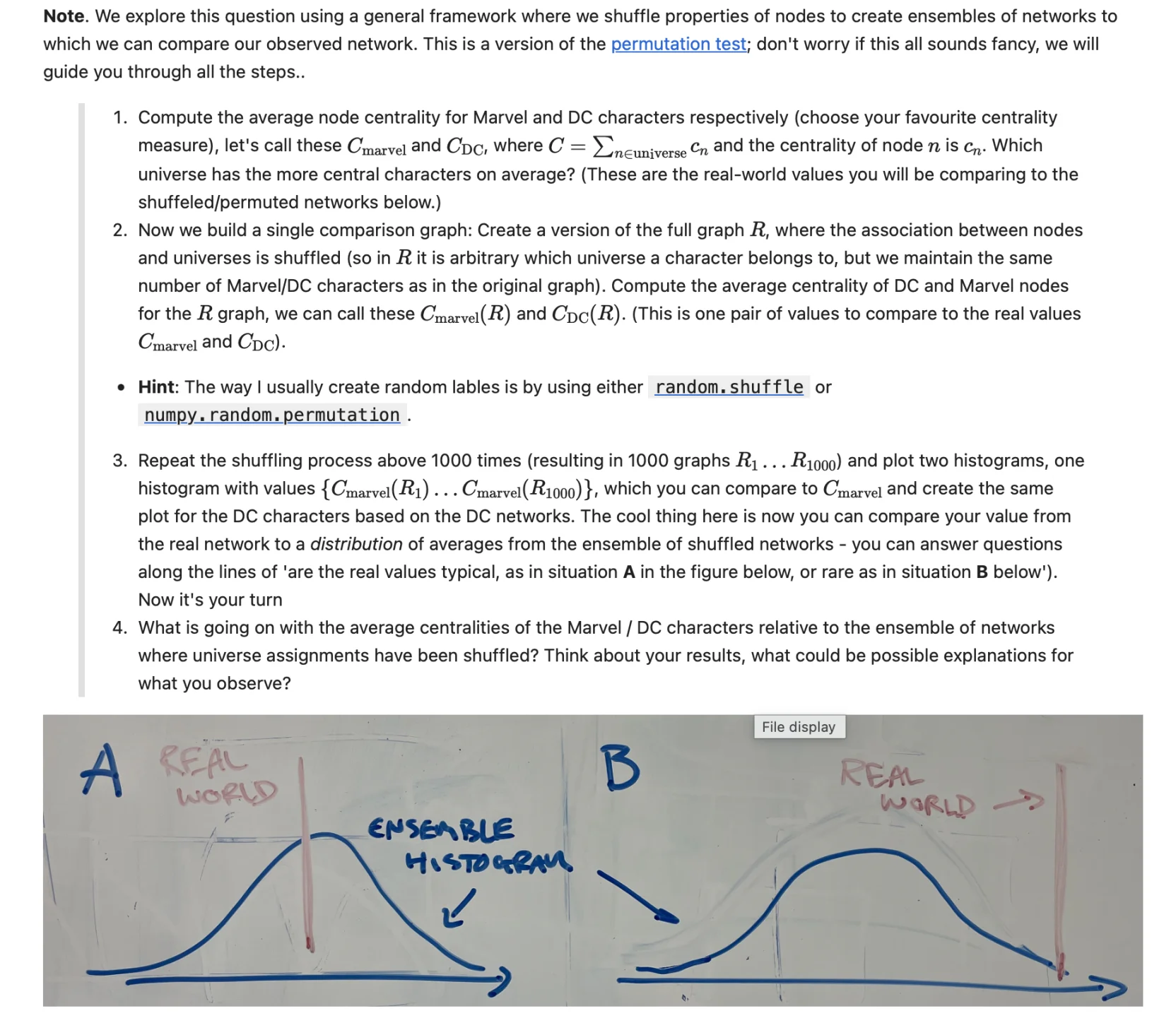
The 2025 version: a notebook exercise (shuffle the Marvel/DC labels, recompute centralities a thousand times) and a whiteboard sketch standing in for the histogram. Situation A is a typical value, situation B is a surprising one. The explorable above draws the real thing.
Read
Network Atlas, Ch. 18 Generating Realistic Data, section 18.1 — the configuration model — and Ch. 19 Evaluating Statistical Significance, section 19.1 Network Shuffling. (19.2 on exponential random graphs is for the curious; it is not on the test.)
2.8 — Compared to what — properly 🧠 Learn + 🔬 Tool
Three short analyses first, each with a flaw in the choice of baseline. For each, name the flaw and the null model that would fix it:
- 🧠 "The Marvel network's average distance (2.7) is no shorter than a random network's (2.8), so it is not a small world."
- 🧠 "39% of links in the directed Marvel network are reciprocated (A links to B and B to A). In a random directed network with the same density only 3% would be, so reciprocity is 13× higher than chance." — what is a better null here, and would the effect survive it? (Think about what the hubs do to reciprocity.)
- 🧠 "Our network's clustering, 0.31, is ten times that of an Erdős–Rényi network, which proves the clustering is caused by the heavy-tailed degree distribution."
- 🚀 Now do it. Load the Marvel network (undirected, giant component), and generate 100 configuration-model networks with its exact degree sequence (
nx.configuration_model, then drop self-loops and parallel links — and report how many links that cost you). Compute $C$ on each. Plot the histogram, draw the real value as a line, report the $z$-score and the empirical $p$-value. Then repeat with 100 random $G(n,m)$ networks and put both histograms on one plot. - 🚀 Same again, but by the other road: start from the real network and apply degree-preserving edge swaps (
nx.double_edge_swap, with many swaps — ten times the number of links is a common rule). Check that the degree sequence really did not change, and compare with the explorable's numbers. Now compare the two roads: the configuration model lands visibly lower than the swaps (around 0.11 versus 0.15). They are supposed to be the same null — so where did the difference come from? (Look at the links you dropped, and at whose links they were.) - 🚀 Now two more quantities: transitivity, and the number of isolated nodes. For each: under which null is the real value unremarkable, and under which is it extreme? What does each answer mean about the network?
- 🧠 Write the paragraph the AI should have written: three sentences that report the clustering result with the right null, the right comparison, and the right conclusion. This is the paragraph that goes in a project paper.
8 · A null model in action: the friendship paradox
Now that we have a null model with any degree distribution we like, there's a cool thing we can test.
You might sometimes feel like your friends have more friends than you do. And — as we will see below — it turns out that it is likely true! This finding is called the friendship paradox.
The intuition in heavy-tailed networks is that you're likely to have a hub as your neighbor. And hubs have so many connections that they bias the average when we calculate the average-number-of-neighbor-friends.
But let's get practical about this. Another way to think about it is that the friendship paradox is a theorem about sampling on networks: picking a random friend of a random person is degree-biased sampling, since a hub is a friend to many and therefore gets picked much more often than a loner.
In the Marvel network, a random character has on average about 10 links; a random neighbor of a random character has about 25. In three out of four samples, the friend is at least as connected as the person.
We can also test that this is true by simply calculating the number. And when we do that, we can phrase it as a null-model question. As you will see below, this time the degree-preserving shuffle does not kill the effect. Only a null that removes the hubs shrinks the effect. But even the random network, as you will see, does not kill the friendship paradox entirely (hint about why in the caption).
Sample 1,000 on the scale-free network and note the two curves, then switch to the random network and ask what changed, and why. The effect doesn't vanish on the random network. Why not? (Hint: even a Poisson has a variance.) Now press Marvel in the explorable above and sample one person at a time: the labels name them. Notice who keeps turning up as "friend" ... and how rarely they turn up as "you."
2.9 — The friendship paradox as a null-model exercise 🧠 Learn + 🔬 Tool
- 🧠 State the paradox precisely: which two averages are being compared, and why is the comparison biased by construction? Then, in one line of algebra: if degrees have mean $\langle k\rangle$ and variance $\sigma^2$, the mean degree of a random neighbor is $\langle k\rangle + \sigma^2/\langle k\rangle$. Use that to explain why the paradox is strongest in scale-free networks and weakest — but not absent — in random ones.
- 🚀 Simulate it on your 5,000-node BA network from 2.5b: sample 1,000 (person, random friend) pairs and report the two mean degrees and the fraction of samples where the friend has at least as many friends. Then on the Marvel network (compare with the numbers on this page). Then on a random network with the same $n$ and $m$ as each.
- 🧠 Null-model it: run the same sampling on a degree-preserving shuffle of the Marvel network. The effect survives — explain why this null cannot kill it, and what that tells you about which network property the paradox really depends on. Then think one step further: could properties beyond the degree sequence (assortativity — do hubs link to hubs? — clustering, communities) make the paradox stronger or weaker? Reason first; test one of them if you can.
- 🔬 Ask your favorite LLM to explain the friendship paradox, then grade its explanation against your simulations and the formula in item 1. Anything subtly wrong, overclaimed, or missing (does it mention the variance? does it say hubs are necessary)? Bring the best wrong sentence to class.
2.10 — Ship an explorable 🚀 Builder · stretch, optional
The widgets on this page are a few hundred lines of vanilla JavaScript each (view source — nothing is hidden). Pick a claim from this week that none of them shows — the four $\langle k\rangle$-regimes of the random network, a configuration model that shows the stubs being paired, what non-linear preference does to the hubs, the friendship paradox as a function of $\gamma$ — and build the explorable that makes it grabbable, agents encouraged, taste yours. The best ones get embedded on this page with credit, and your group gets a permanent place in the course.
2.11 — Go nuts with your LLM 🚀 Builder · every week
The standing rules live in week 1, exercise 1.8: one free-form post on your group's site, on the shared Marvel network, link in this week's Teams channel by Monday evening, friendly criticism for at least one other group. Winner announced at 09:00 next Wednesday.
This week you have models and null models. Some openers, if you want them:
- Does the real network's degree distribution look more random, more BA, or neither? Make the case with a CCDF and a fit — and say what you can't conclude.
- Does the friendship paradox hold among superheroes — who are the "popular friends" that drive it? Is there a character nobody is out-popularityed by?
- Pick any number you can compute on the network — reciprocity, triangles, the number of islands, the biggest hub's share of all links, anything — and shuffle-test it (the explorable does five; you can do any). Which properties survive a degree-preserving shuffle, and which die? Tell us what the survivors mean.
- Grow your own Marvel: run preferential attachment to $n = 303$, $m$ tuned to match, and put it next to the real thing. What does the model get right, and what is the most glaring thing it gets wrong?
- Or ignore all of this and chase whatever the explorables made you wonder about — the winner is rarely the group that played it safe.
Standing option, weeks 2–4: crawl a different Wikipedia category of your own choosing (the API notes are in week 1) and run this week's toolkit there instead. Good rehearsal — your final project will live on a domain you pick.
Essentials
The 🧠 Learn core of the week: the models, the numbers each one predicts, and the test that turns a model into a null. All of it is pen-and-paper material — if a line below feels shaky, the section that teaches it is one click up the page.
- Erdős–Rényi random network $G(n,p)$
- every one of the $n(n-1)/2$ possible pairs is linked independently with probability $p$. Expected number of links $p\,n(n-1)/2$; expected degree $\langle k\rangle = p(n-1)$; clustering $C = p$.
- Poisson degree distribution
- what the sparse random graph's degrees follow — concentrated near $\langle k\rangle$, tails dying fast. No hubs.
- Giant component (random graph)
- appears at $\langle k\rangle = 1$ — below it, islands; above it, one component swallows almost everything.
- Six degrees (short paths)
- distances in real networks are tiny — and chance agrees: reach multiplies by $\langle k\rangle$ per step, so a random network is $d \approx \ln n / \ln\langle k\rangle$ hops across. Growing like $\log n$ = short. Short paths are not evidence against randomness.
- Local clustering coefficient
- $C_i = 2e_i/[k_i(k_i-1)]$ — the fraction of pairs of $i$'s neighbors that are themselves linked ($e_i$ links among $k_i(k_i-1)/2$ possible pairs). Set to $0$ when $k_i < 2$.
- Average clustering $C$ · transitivity
- $C$ is the mean of $C_i$ over all nodes; transitivity counts triangles over the whole network at once. They differ when hubs and low-degree nodes live in differently tight neighborhoods.
- Lattice
- every node linked to its nearest neighbors — all clustering, but distances grow like $n$.
- Small world
- clustering far above chance and distances at chance ($\sim \log n$). Real networks have both; the random graph and the lattice each have only one.
- Watts–Strogatz model
- a lattice with a small fraction $q$ of links rewired into shortcuts. A handful of shortcuts collapse the distances while barely touching the clustering.
- Power law
- $P(k) \sim k^{-\gamma}$ — a straight line on log–log axes, no typical scale, and hubs neither chance nor shortcuts can make.
- Preferential attachment (Barabási–Albert)
- real networks grow, and newcomers link to node $i$ with probability $\Pi(k_i) = k_i / \sum_j k_j$. Growth and preference together give a power law with $\gamma = 3$; neither alone does.
- CCDF
- the complementary cumulative distribution — for each $k$, the fraction of nodes with degree at least $k$. Tames tail noise with no binning at all.
- Null model
- a model used not as a hypothesis about the world but as a baseline for "nothing interesting going on." Choosing the null changes the conclusion, not just the number.
- Configuration model
- the random network with exactly the real degree sequence — give every node its real degree in "stubs," pair the stubs uniformly at random.
- Degree-preserving shuffle
- rewire A–B and C–D into A–D and C–B, thousands of times. Every node's degree survives; who-links-to-whom is scrambled. The practical route to the configuration model.
- Shuffle test
- shuffle many times and your statistic gets a distribution under the null. Report the $z$-score (standard deviations between the real value and the shuffle mean) and the empirical $p$-value (fraction of shuffles at least as extreme). A permutation test by another name.
- Friendship paradox
- a random neighbor of a random node has mean degree $\langle k\rangle + \sigma^2/\langle k\rangle$ — at least $\langle k\rangle$, because picking a friend is degree-biased sampling. Its strength is set by the degree variance.
On Test 1
From this week, you should be able to do the following on paper, closed book. Any formula you need is printed on the test paper — you are never asked to write one from memory:
- for a random network $G(n,p)$: compute the expected number of links, the expected degree, and $C$; know that its degree distribution is Poisson (no hubs), that its giant component appears at $\langle k\rangle = 1$, and why its distances are short ($\langle k\rangle^d \approx n$ gives $d \approx \ln n/\ln\langle k\rangle$);
- compute a local clustering coefficient on a small example, and the network average; say what transitivity measures instead and when the two differ;
- explain the small-world signature (clustering far above chance, distances at chance) and the mechanism by which a few shortcuts collapse distances without touching $C$;
- identify a model (random / Watts–Strogatz / Barabási–Albert / lattice) from a plotted or described degree distribution or a described property — and say what would break if the axes changed;
- predict how $C$, $\langle d\rangle$ and the giant component respond when $n$, $\langle k\rangle$, $p$ or $m$ change;
- compute a degree-proportional attachment probability from a list of degrees; explain why growth and preference are both needed for hubs, and why early nodes win;
- read a log–log plot honestly: say what a straight line does establish (a heavy tail) and what it does not (a power law with a particular $\gamma$); know what the CCDF is and why it needs no binning;
- explain what a degree-preserving shuffle keeps and what it destroys; choose the right null model for a claim — and spot the flaw in a short (possibly AI-written) analysis that compares against the wrong one, e.g. using a random-network baseline to attribute an effect to the degree distribution;
- read a shuffle-test figure: a histogram of shuffled values with the real value marked — and say what the $z$-score and the empirical $p$-value mean;
- state the friendship paradox precisely and name the one network property that determines how strong it is.
Goodies
Everything above is the course. Everything below is for the student who finished the page and wants more. Nothing here is on the test; all of it is worth your time.
For the one student who wants the random-graph mathematics
Everything Part 2 asserted, derived. A node in $G(n,p)$ has $n-1$ potential links, each present with probability $p$, so its degree is binomial: $P(k) = \binom{n-1}{k} p^k (1-p)^{n-1-k}$, with mean $\langle k\rangle = p(n-1)$ and variance $p(1-p)(n-1) \approx \langle k\rangle$ for sparse networks.
Two limits. Let $n \to \infty$ with $\langle k\rangle$ fixed (so $p \to 0$ — the sparse limit, which is the one real networks live in) and the binomial becomes the Poisson distribution, $P(k) = e^{-\langle k\rangle}\langle k\rangle^k / k!$: it depends on $\langle k\rangle$ alone, not on $n$, which is why a random network with a million nodes and one with a thousand have the same degree distribution if their average degrees agree. Now let $\langle k\rangle$ itself grow large and the Poisson becomes a normal distribution with mean and variance both $\langle k\rangle$ (de Moivre–Laplace, or just the central limit theorem: a degree is a sum of many coin flips). Either way the tail falls off faster than any power law — the probability of a node with degree $10\langle k\rangle$ is astronomically small. This is the precise sense in which "a random network has no hubs."
Isolates and connectivity. A node is isolated with probability $P(0) = e^{-\langle k\rangle}$, so the expected number of isolates is $n\,e^{-\langle k\rangle}$; setting it to 1 gives the threshold $\langle k\rangle = \ln n$ at which the network typically becomes fully connected.
The giant component. Let $S$ be the fraction of nodes in the giant component. A node is outside it only if none of its $\langle k\rangle$ neighbors are inside, which gives the self-consistent equation $1 - S = e^{-\langle k\rangle S}$. It has a non-zero solution only for $\langle k\rangle > 1$ — that is the phase transition — and $S$ rises steeply just above it. The curve in the explorable is this equation.
The four regimes, as Barabási names them: subcritical ($\langle k\rangle < 1$: fragments of size $\sim \ln n$), critical ($\langle k\rangle = 1$: the largest component scales as $n^{2/3}$), supercritical ($\langle k\rangle > 1$: one giant component plus small fragments), connected ($\langle k\rangle > \ln n$: no isolates).
Distances. A node reaches $\langle k\rangle$ nodes in one step, roughly $\langle k\rangle^2$ in two, $\langle k\rangle^d$ in $d$ — so it has reached everyone when $\langle k\rangle^d \approx n$, i.e. $\langle d\rangle \approx \ln n / \ln\langle k\rangle$. For Marvel that is $\ln 303 / \ln 9.5 \approx 2.5$, close to the measured 2.8.
Clustering. $C = p = \langle k\rangle/(n-1)$, which for fixed $\langle k\rangle$ vanishes as $1/n$. Real networks have $C$ that does not depend on $n$ at all — the cleanest single statement of what the random graph is missing.
Why the physicists went wild: power laws, universality, and renormalization
It is hard to understand from outside why a straight line on a log–log plot caused such a stir in 1999. Here is the reason, and it is a beautiful one.
In the 1960s and 70s physics solved one of its great puzzles: what happens at a critical point — water at the exact temperature and pressure where liquid and vapour become indistinguishable, a magnet at the exact temperature where it loses its magnetism. At a critical point every quantity you can measure becomes a power law in the distance from the point, and the system looks the same at every scale: zoom in on a picture of the fluctuations and you cannot tell how far you zoomed. That is scale invariance, and a power law is the only function with the property that stretching its argument only rescales it: $f(ax) = a^{-\gamma} f(x)$. Ken Wilson's renormalization group (Nobel Prize, 1982) explained it: at criticality the microscopic details wash out under repeated coarse-graining, and what survives — the exponents — depends only on a few gross features like dimensionality and symmetry. This is universality: wildly different systems (a fluid, a magnet, a binary alloy) share exactly the same exponents, because they sit in the same universality class. The exponents are, in a precise sense, the deepest thing you can know about a system, and measuring one is measuring its class.
Now put yourself in the shoes of a statistical physicist in 1999 — Barabási trained with Gene Stanley, one of the architects of this programme. You plot the degree distribution of the web and see a power law. The entire apparatus fires at once: no characteristic scale (hence "scale-free"); a mechanism so simple it might be universal; the dream that $\gamma$ sorts real networks into universality classes, so that measuring one exponent tells you which class the internet, the cell and society belong to. That is why so many papers in 2000–2005 reported one thing — an exponent — and why the physicists could not stop; and why the growth-and-preference mechanism was such a satisfying answer (Barabási's model sits right in this tradition: a few ingredients, a power law out).
The dream only partly came true. Measured exponents scatter between 2 and 3 and beyond, with no sign of clean classes; many different mechanisms produce power laws (preferential attachment was itself rediscovered — Yule 1925, Simon 1955, Price 1976 got there first, in other fields); and as the next box explains, many of the reported power laws were never really there. What remains is real and important: heavy tails, hubs, the absence of a typical scale, and a way of thinking — mechanism first, ask what is universal — that the field would not have without them. Watts and Strogatz were a mathematician and a sociologist-in-training; the scale-free story is the physicists' contribution to network science, for better and for worse.
How to fit a power law — and how the field got it wrong for a decade
For about ten years the standard method was: histogram the degrees, plot on log–log axes, fit a straight line by least squares, report the slope as $\gamma$. Nearly every early paper did it, and it is wrong in at least four ways. The fit is dominated by the few noisy points in the tail (where every count is 0 or 1) or, if you bin, by your binning choices; least squares on log-transformed counts is biased, so the slope is systematically off; a straight line fit gives you no way of asking whether a power law is the right model at all; and the usual "$R^2 = 0.98$" is meaningless, because smooth heavy-tailed alternatives like the log-normal give equally straight lines over the two or three decades of data most networks have. Goldstein, Morris & Yen pointed this out in 2004; Newman's Power laws, Pareto distributions and Zipf's law (2005) is the gentle introduction to the right mathematics.
The method that replaced it is Clauset, Shalizi & Newman, Power-law distributions in empirical data (2009), and it has three steps. (1) Estimate $\gamma$ by maximum likelihood, not by a line: for a discrete power law starting at $k_{\min}$ the estimate is approximately $\hat\gamma = 1 + n \left[\sum_i \ln \frac{k_i}{k_{\min} - 1/2}\right]^{-1}$ — no histogram, no bins, an honest standard error. (2) Choose $k_{\min}$ — the point where the power law starts (there is almost always a bend at small $k$) — by picking the value that makes the fitted CCDF closest to the empirical one (the Kolmogorov–Smirnov distance). (3) Test it: generate many synthetic datasets from the fitted power law, fit each one the same way, and ask how often the synthetic data fits worse than the real data did — a $p$-value for "a power law is a plausible model" (note the direction: a small $p$ rejects the power law). And then, whatever the $p$, compare against alternatives with a likelihood-ratio test — log-normal, exponential, power law with cut-off — because "plausible" is not "best." The Python package powerlaw implements all of it in a few lines.
When Broido & Clauset ran this on nearly a thousand real networks (Scale-free networks are rare, 2019), only a small minority passed the strict test and a log-normal fit most of them as well or better. The preprint made the news (Quanta, then The Atlantic), and Barabási answered within weeks with a blog post that is a genuinely fun read: Love is All You Need: Clauset's fruitless search for scale-free networks (March 2018). His argument: the theory never predicted pure power laws in real networks — growth plus preferential attachment plus any realistic extra ingredient (internal links, aging, fitness) predicts a power law with corrections, so fitting a pure power law to 927 networks and finding few of them tests a straw man; and the strict test is so strict that it fails the BA model itself. The one-liners are worth the visit (a box on searching for the word "Love" in the string "Love," and a rock and a feather dropped from his office window to disprove Newton). Read it as a partisan document, which it is; the technical version of the same side is Voitalov et al. 2019 (finite networks with cut-offs are still "scale-free" in the sense that matters), and Holme's Rare and everywhere is the balanced summary (Petter Holme is also an episode of my podcast, with Gourab Ghoshal, on a 2006 paper about agents competing for centrality): heavy tails are everywhere; power laws in the strict sense are rare; and the practical consequences of a heavy tail — hubs, the friendship paradox, epidemics that will not die — do not depend on which of the two you have. Do the exercise 2.6 paragraph with that in mind.
Shuffling is a permutation test
If you have taken a statistics course, Part 7 should feel familiar. In 1935 Ronald Fisher described a lady who claimed she could tell whether the milk or the tea had been poured first; the test he proposed was to enumerate every way her eight answers could have been assigned by chance and ask how extreme her actual answers were among them. That is a permutation test: instead of assuming a formula for the null distribution, you build it by rearranging the data in every way consistent with "nothing going on," and you locate the real value in the pile. The logic rests on exchangeability — under the null, the rearranged datasets are just as likely as the real one.
Network shuffling is exactly this, with one twist: the "rearrangements consistent with nothing going on" are the networks with the same degree sequence, and there are far too many to enumerate, so we sample a few hundred of them. Everything else carries over, including the pitfalls. The $z$-score assumes the shuffled values are roughly normal — true for global averages like $C$ by the central limit theorem, and visibly false for some quantities (the number of isolates, say), so always look at the histogram before quoting a $z$. The empirical $p$-value should be computed as $(1 + \text{number of shuffles at least as extreme}) / (1 + \text{number of shuffles})$, so that 200 shuffles can never give you $p = 0$; and if you test twenty quantities you will find one "significant" at $p < 0.05$ by construction. Decide one-sided or two-sided before you look. And make sure the shuffle has actually mixed: too few edge swaps leave the network close to the original, and the null looks suspiciously like reality.
The degree-preserving version was made standard in network science by Maslov & Sneppen (Specificity and stability in topology of protein networks, Science 2002) and by Milo et al.'s network motifs the same year — the idea of counting small subgraphs and asking which ones are over-represented relative to the shuffle, which is the null-model habit in its purest form. Everything in week 4 (communities, backbones) will quietly rest on the same logic.
The three papers that started it. The models above are each a single short paper, and all three are readable in an evening. Watts & Strogatz, Collective dynamics of 'small-world' networks (Nature, 1998 — four pages, one figure, the one you reproduced in 2.4). Barabási & Albert, Emergence of scaling in random networks (Science, 1999 — growth plus preferential attachment, three pages). And the grand-daddy, Erdős & Rényi, On the evolution of random graphs (1960) — the phase transition, proved; harder going, but the Atlas and Barabási both retell it.
Barabási's own version. Last year's textbook, Network Science, tells this week's story as a narrative in three chapters: Ch. 3 Random Networks (the four regimes of $\langle k\rangle$, and the "small world" argument in 3.8–3.9), Ch. 4 The Scale-Free Property (what $\gamma$ does — the three regimes of section 4.7 are worth knowing), Ch. 5 The Barabási–Albert Model (including 5.7–5.8 on what happens when the preference is non-linear: sub-linear gives stretched exponentials, super-linear gives one winner-takes-all node). It is the model-first telling by the person who started the argument; the Atlas is the encyclopedic one. Read both and notice where they disagree about how much power laws matter.
The friendship paradox, original and applied. Scott Feld, Why your friends have more friends than you do (1991) is the sociology paper that named it. The applied side is beautiful: because a random friend is a hub-biased sample, monitoring friends of random people detects an epidemic earlier than monitoring random people — Christakis & Fowler (2010) did exactly this with flu on a college campus. Same theorem, used as an instrument. The one-line version: the mean degree of a random neighbor is $\langle k^2\rangle / \langle k\rangle$, which exceeds $\langle k\rangle$ whenever the variance is positive — and for a power law with $\gamma \leq 3$ the variance diverges, so in a large scale-free network your friends have, on average, infinitely more friends than you.
A harder friendship-paradox exercise, from an earlier year. What if the power law is flatter — $\gamma = 2$ instead of 3? Reason first: flatter means more and bigger hubs, so the paradox should be stronger. Then test it: generate a 5,000-node degree sequence from a power law with exponent 2 using the transformation method (Newman 2005, section 2: $x = x_{\min}(1-r)^{-1/(\alpha-1)}$ for uniform $r$; round to integers; make the sum even), feed it to nx.configuration_model, and measure the paradox as in 2.9. Then do the same with $\gamma = 3$ and compare against your BA network — same degree distribution, different generating process. Are they different? How would you test that rigorously (error bars, a test)?
Playable versions. Nicky Case's The Wisdom and/or Madness of Crowds (also in week 1's Goodies) contains a hands-on small-world builder and the majority illusion — the friendship paradox's cousin, where a few well-placed hubs make a rare opinion look like the majority. And Veritasium's six-degrees video is the popular telling of Part 5.